
Three level transmitters. Two-out-of-three voting. Any single transmitter can fail and the trip still works. It feels like the safest sensor arrangement on the P&ID, and against independent failures it nearly is. Then you add one modest assumption, that 5% of dangerous failures hit all three channels together, and the calculated PFDavg gets 48.5 times worse. This paper builds the model that shows why, step by step, and checks it against an independent closed-form solution.
The paper in 60 seconds
- States are engineering decisions. Keep a state only if it changes demand success, diagnostics, repair or test response.
- A proof test is scheduled, not random. A plain Markov chain is memoryless, so the test is applied as a separate reset.
- Redundancy kills independent failures but leaves a common-cause floor. That floor usually decides the number.
- Exact maths can still be wrong for the plant if data boundaries, coverage, repair policy or dependencies are wrong.
- PFDavg is one gate of three. Architecture and systematic capability remain separate requirements.
1. Why reach for a Markov model at all?
For a single unrepaired channel, the familiar shortcut is PFDavg ≈ λDU × T / 2. It is good when its assumptions hold and the failure probability is small.
Once voting, diagnostics, repair and common causes enter, the shortcut hides more than it shows. A Markov chain does the opposite. It lists every state the system can be in and tracks how probability moves between them over time, so every assumption sits in plain view as a state or an arrow.
That is not a claim that Markov always beats fault trees, reliability block diagrams or formulas. The rule is simpler: use the simplest method that captures the dependencies and time behaviour your decision depends on.
2. Five states are enough
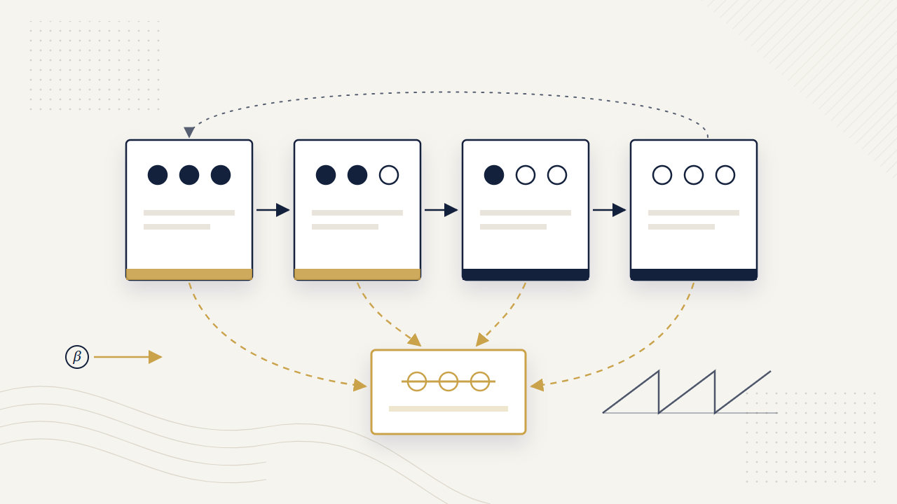
Track the 2oo3 group by how many channels have failed dangerously and undetected since the last proof test: 0, 1, 2 or 3. Add one more state, C, for a common-cause event that takes out the whole group at once. With two or more channels gone, or in C, the group cannot act on a demand.
The worked numbers: λDU = 60 FIT per channel (1 FIT = 10−9 failures per hour) and β = 5%. The β-factor splits each channel's rate into an independent part λi = (1 − β) λDU = 57 FIT and a group-wide common-cause rate λc = β λDU = 3 FIT.
| From | To | Rate | Why |
|---|---|---|---|
| 0 | 1 | 3λi | Any of three healthy channels can fail |
| 1 | 2 | 2λi | Two healthy channels remain |
| 2 | 3 | λi | The last channel fails |
| 0, 1, 2, 3 | C | λc | One shock disables the group |
C is absorbing until the next test. Treating common cause as one group-wide shock is deliberately simple; real systems may need partial common-cause groups.
3. The whole method in two lines
Put the state probabilities in a row vector p(t) and the transition rates in a generator matrix Q. Each off-diagonal entry is a rate and each row sums to zero. Then:
Mark the dangerous states with a reward vector r = [0, 0, 1, 1, 1]. The instantaneous unavailability is p(t)·r, and the number we report is its average over the test interval:
4. Solve it twice, from two directions
A result is only as credible as its cross-check. For this model there is an independent route that never mentions a matrix. A surviving channel has failed by time t with probability q(t) = 1 − e−λit, and a common-cause shock has occurred with probability c(t) = 1 − e−λct. The group succeeds only if no shock occurred and at least two channels survive:
Averaged over T, with A(a,T) = (1 − e−aT)/(aT):
The state-space answer and the event-based answer must agree for identical assumptions. If they do not, one of them is wrong. (In software, evaluate small aT with expm1 to avoid cancellation.)
5. The result
| Method / scenario | PFDavg |
|---|---|
| Markov chain (CTMC), β = 5% | 1.338904489e−5 |
| Independent closed form, β = 5% | 1.338904489e−5 |
| No common-cause mechanism (β = 0) | 2.760739324e−7 |
| Common-cause shock alone | 1.313988489e−5 |
The two methods agree to numerical precision. Look at the last row: the common-cause shock on its own is 1.314 × 10⁻⁵, almost the entire answer. The redundancy is doing its job against independent failures. It just cannot touch the failure that hits all three channels together.
6. The 5% that decides everything
Hold each channel at 60 FIT and change only β. The result is nearly a straight line: PFDavg is governed by the common-cause assumption far more than by the voting.
| β | 0% | 1% | 3% | 5% | 10% | 20% |
|---|---|---|---|---|---|---|
| PFDavg | 2.761e−7 | 2.899e−6 | 8.144e−6 | 1.339e−5 | 2.650e−5 | 5.273e−5 |
Now the surprise. With the same data, here is how three architectures compare over one year:
| Architecture | PFDavg | What has to happen |
|---|---|---|
| 1oo1 | 2.628e−4 | The one channel fails |
| 1oo2 | 1.322e−5 | Both channels fail, or a group-wide common cause |
| 2oo3 | 1.339e−5 | Two of three fail, or a group-wide common cause |
1oo2 and 2oo3 land within 1.3% of each other, because the shared common-cause floor dominates both. That says nothing about spurious trips, diagnostics or operating preference, which need their own models. It does say that adding a third transmitter does not buy dangerous-failure performance while the common cause stays where it is.
Try it: move β and watch the floor
This uses the paper's closed form for a DU-only group with a perfect proof test. It is for building intuition, not for a SIL claim.
7. From a maths model to a plant model
The worked example is deliberately clean. A real SIF needs more, and each item below changes the model, not just the numbers.
Detection and repair
A dangerous detected failure might trip the plant, call maintenance, or leave the function running impaired under compensating measures. Those are different states. Repair can be a rate μ = 1/MTTR where that approximation is defensible; separate detection time, administrative delay, hands-on repair and restoration testing where they matter.
Imperfect and partial proof tests
Model the test as a state-transfer matrix R at t = T. A perfect test sends everything back to healthy. An imperfect one must keep the probability in failure modes it cannot reveal. Resetting everything would understate PFDavg. Partial tests may need multi-phase models.
Dependence is wider than one β
Shared impulse lines, calibration methods, power supplies, environment, design defects and maintenance practice are all coupling mechanisms. A constant β is a transparent approximation, not a physical explanation, so record the boundary and source behind it.
What a plain Markov chain cannot do
Fixed test dates, fixed repair durations, wear-out and demand damage break the memoryless assumption. Piecewise or phased models, semi-Markov methods, age states or Monte Carlo simulation are the remedies. More states do not fix the wrong stochastic assumptions.
8. A review checklist you can use on Monday
Credibility comes from checks anyone can repeat, not from the complexity of a diagram. Before a Markov result goes into a report, confirm:
- Probability is conserved: p(t) sums to one and every state stays within [0, 1].
- The generator is valid: Qij ≥ 0 off the diagonal and each row sums to zero.
- Boundaries behave: PFD(0) = 0 after a perfect test, and β = 0 reproduces independent voting.
- A second method agrees: closed form or numerical integration matches the chain.
- Sensitivities point the right way: a longer test interval or higher β never improves the result.
- The reset is honest: perfect tests reset covered states; imperfect tests keep uncovered ones.
- Data is traceable: channel boundary, failure-rate category, source version, units and β meaning are recorded.
- Numerics are controlled: solver tolerance and integration convergence are stated.
- The claim is separated: a PFDavg pass is not reported as architectural or systematic compliance.
For this benchmark, the chain and the closed form differ by less than 10−12 in absolute PFDavg. That checks the mathematics of the example; it is not evidence about any particular software implementation.
9. Leave a record another engineer can rerun
"We used a Markov model" is not a calculation record. The minimum is the state dictionary, the transition table, Q, initial conditions, the demand-failure reward, the reset policy, the analysis horizon, the integration method, parameter sources and the numerical checks. With those, anyone can rebuild the result: assemble the 5 × 5 generator, evaluate p(0)exp(Qt), sum states 2, 3 and C, average over 8,760 h, and compare with the closed form.
10. The takeaway
A Markov result is not credible because it uses matrices. It is credible when the physical model, parameter meanings, transitions, test policy and validation all survive review. The 2oo3 example teaches three things: redundancy suppresses independent simultaneous failures; a modest common-cause assumption can dominate what is left; and an independent cross-check can test a model before anyone relies on it.
Inside the IEC 61508 / IEC 61511 lifecycle, Markov modelling adds rigour to quantitative SIL verification. It does not replace risk allocation, architectural constraints, systematic integrity, field evidence or independent review. For how those fit together, read The Three Gates to SIL.
Abbreviations and symbols
| CCF | Common-cause failure |
| CTMC | Continuous-time Markov chain |
| DD / DU | Dangerous detected / dangerous undetected failure |
| FIT | Failures in time: 10−9 failures per hour |
| PFDavg | Average probability of dangerous failure on demand |
| β | Beta factor (simplified common-cause allocation) |
| λi / λc | Independent channel / group common-cause failure rate |
| Q / r | Generator matrix / demand-failure reward vector |
| T | Proof-test interval |
- IEC 61511-1:2016+AMD1:2017, Functional safety: safety instrumented systems for the process industry sector, Part 1.
- IEC 61508-6:2010, Guidelines on the application of IEC 61508-2 and -3.
- Innal, F., Lundteigen, M.A., Liu, Y., Barros, A. (2016). PFDavg generalized formulas for SIS subject to partial and full periodic tests based on multi-phase Markov models. Reliability Engineering & System Safety 150, 160–170. doi:10.1016/j.ress.2016.01.022
- Ottermo, M.V., Hauge, S., Håbrekke, S. (2021). Reliability Data for Safety Equipment: PDS Data Handbook, 2021 Edition. SINTEF Digital.
- Trivedi, K.S., Ciardo, G., Malhotra, M., Sahner, R.A. (1993). Dependability and performability analysis. NASA-CR-191565.
- IEC 61508-2:2010, Requirements for E/E/PE safety-related systems.
- Butler, R.W. (1985). An Abstract Specification Language for Markov Reliability Models. NASA TM-86423.